In late September I started a project on Dgraph, that I planned to finish on parental leave. Fast-Forward to today: 2019 and my parental leave are almost over.
Software Estimations are easy!
I noticed, that I am not making any progress with the Dgraph project. The problem of building an interesting dataset and at the same time learning about Dgraph turned out to be a little too ambitious.
So I started to learn about "classic" Triplestores and Semantic Web Technologies first:
My idea was to build the dataset by implementing the parsers one by one and more importantly I wanted to get a feeling how RDF and SPARQL works. I have learned a lot along the way and best of it all, I now have a RDF dataset for Dgraph.
You can find all code and a guide on how to build the datasets in my GitHub Repository at:
So what is DGraph?
According to the official documentation Dgraph is:
[...] an open source, scalable, distributed, highly available and fast graph database, designed from ground up to be run in production.
About this Project
Every project starts with an idea. I have worked with weather data and airline data in the past, so the idea is to use a Dgraph to query Aviation data, using information from:
- Aircrafts
- Airports
- Carriers
- Flights
- Weather Stations
- ASOS / METAR Weather Data
You can find all code and a guide on how to build the datasets in my GitHub Repository at:
What this Project is about
In the internet you seldomly get an idea how to really read, transform, import and query data. Often enough the datasets are prepared for you and it's hard to get an idea how to merge datasets and build import pipelines.
This project shows how to:
- Create an RDF dataset from multiple data sources
- Bulk Import an RDF Dataset to Dgraph
- Query the Data using the Dgraph GraphQL query language
What this Project is not about
It's not an introduction.
The Dgraph team puts a lot of effort into the documentation, and it is the best place to get started:
I highly suggest to take the Tour of Dgraph:
It's not about benchmarks.
My past articles on Graph Databases focused on the performance of database systems (see articles on SQL Server 2017 and Neo4j).
These comparisms are often unfair and very misleading.
Why was the SQL Server 2017 Graph Database so fast? Because its Columnstore compression algorithms make it possible to fit the entire dataset into RAM. Once the datasets get bigger and systems hit the SSD / HDD, we will see very different results.
Fair benchmarks are hard to create and this article intentionally doesn't compare systems anymore.
Datasets
In this article I will use several open datasets and show how to parse and import them to a Dgraph database. I am
unable to share the entire dataset, but I have described all steps neccessary to reproduce the article in the
subfolders of /Dataset/Data.
I am using data from 2014, because this allows me to draw conclusions against the following previous Graph Database articles:
- Learning Neo4j at Scale: The Airline On Time Performance Dataset
- Analyzing Flight Data with the SQL Server 2017 Graph Database
Airline On Time Performance (AOTP)
Is a flight delayed or has been cancelled? The National Transportation Safety Board (NTSB) provides the so called Airline On Time Performance dataset that contains:
[...] on-time arrival data for non-stop domestic flights by major air carriers, and provides such additional items as departure and arrival delays, origin and destination airports, flight numbers, scheduled and actual departure and arrival times, cancelled or diverted flights, taxi-out and taxi-in times, air time, and non-stop distance.
The data spans a time range from October 1987 to present, and it contains more than 150 million rows of flight informations. It can be obtained as CSV files from the Bureau of Transportation Statistics Database, and requires you to download the data month by month:
More conveniently the Revolution Analytics dataset repository contains a ZIP File with the CSV data from 1987 to 2012.
ASOS / AWOS Weather
Is a flight delayed, because of weather events? Many airports in the USA have so called Automated Surface Observing System (ASOS) units, that are designed to serve aviation and meterological operations.
The NOAA website writes on ASOS weather stations:
Automated Surface Observing System (ASOS) units are automated sensor suites that are designed to serve meteorological and aviation observing needs. There are currently more than 900 ASOS sites in the United States. These systems generally report at hourly intervals, but also report special observations if weather conditions change rapidly and cross aviation operation thresholds.
ASOS serves as a primary climatological observing network in the United States. Not every ASOS is located at an airport; for example, one of these units is located at Central Park in New York City. ASOS data are archived in the Global Surface Hourly database, with data from as early as 1901.
But where can we get the data from and correlate it with airports? The Iowa State University hosts an archive of automated airport weather observations:
The IEM maintains an ever growing archive of automated airport weather observations from around the world! These observations are typically called 'ASOS' or sometimes 'AWOS' sensors. A more generic term may be METAR data, which is a term that describes the format the data is transmitted as. If you don't get data for a request, please feel free to contact us for help. The IEM also has a one minute interval dataset for Iowa ASOS (2000-) and AWOS (1995-2011) sites. This archive simply provides the as-is collection of historical observations, very little quality control is done. "M" is used to denote missing data.
The Iowa State University also provides a Python script to download the ASOS / AWOS data:
NCAR Weather Station List
What type of weather station are the measurements from? What is the name of the weather station? What is its exact location?
We could compile a list of stations from files in the Historical Observing Metadata Repository:
But while browsing the internet I found a list of stations, that contains all information we need. And I am allowed to use it with the permission of the author. I uploaded the latest version of June 2019 into my GitHub repository, because I needed to make very minor modifications to the original file:
FAA Aircraft Registry
Which aircraft was the flight on? Which engines have been used?
Every airplane in the world has a so called N-Number, that is issued by the Federal Aviation Administration (FAA).
The FAA maintains the Aircraft Registry Releasable Aircraft Database:
[...]
The archive file contains the:
- Aircraft Registration Master file
- Aircraft Dealer Applicant file
- Aircraft Document Index file
- Aircraft Reference file by Make/Model/Series Sequence
- Deregistered Aircraft file
- Engine Reference file
- Reserve N-Number file
Files are updated each federal business day. The records in each database file are stored in a comma delimited format (CDF) and can be manipulated by common database management applications, such as MS Access.
It is available at:
I have used some Excel-magic to join the several files into one and export a CSV File, that strips all sensitive data off and could be parsed easily:
Parsing the Datasets
In this section we will take a look at how to go from many CSV files to a Dgraph-compatible RDF file.
From CSV to .NET
A lot of datasets in the wild are given as CSV files. Although there is a [RFC 4180], the standard only defines the structure of a line in the CSV data (think of newline characters, delimiters, Quoted Data, ...).
A CSV file doesn't have something like defined formats, think of:
- Date formats
- Culture-specific formatting
- Text Representation of missing values
- Text Representation of duration (Milliseconds, Seconds, Minutes, ...)
- ...
In any data-driven project most of the time goes into:
- Analyzing
- Preprocessing
- Normalizing
- Parsing
To simplify and speed up CSV parsing I wrote TinyCsvParser some years ago. As a library author it's important to eat your own dogfood and it makes good example to show how I would approach such data.
Basically I structure the CSV parsing for every dataset in its own project, like this:
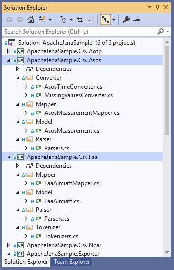
This leads to a nice separation of concerns:
- Converter
- Provides Converters to parse Dataset-specific values / formats
- Mapper
- Defines the Mapping between the CSV File and the C# Domain Model
- Model
- Contains the C# Domain Model
- Parser
- Provides the Parsers with information about:
- Should the header be skipped?
- Which Column Delimiter should be used?
- Which Mapping should be used?
- Provides the Parsers with information about:
- Tokenizer
- Defines how to tokenize the CSV data:
- Is a
string.Split(...)sufficient for the data (saves CPU cycles)? - Is it a fixed-width format?
- Is a
- Defines how to tokenize the CSV data:
From .NET to RDF
There is a great .NET library for working with all kinds of RDF data called dotNetRDF:
The dotNetRDF website writes:
dotNetRDF is...
- A complete library for parsing, managing, querying and writing RDF.
- A common .NET API for working with RDF triple stores such as AllegroGraph, Jena, Stardog and Virtuoso.
- A suite of command-line and GUI tools for working with RDF under Windows
- Free (as in beer) and Open Source (as in freedom) under a permissive MIT license
While very advanced and complete, I need dotNetRDF primarly for writing RDF data. In my article on Apache Jena I have already created a RDF dataset for Aviation data. The idea was to use the same RDF dataset.
RDF Types
Dgraph supports the following set of RDF types:
So for the RDF data I removed all occurences of xs:durations, and turned the values into xs:dateTime.
Predicates and URIs
The original dataset represented the serial number of an Aircraft like this:
<http://www.bytefish.de/aviation/Aircraft#NW8172> <http://www.bytefish.de/aviation/Aircraft#serial_number> "123"^^<http://www.w3.org/2001/XMLSchema#string>
In RDF all predicates are given as IRI (an extension of a URI), but I don't want full URIs as predicate names in Dgraph. Why? It would lead to ugly & hard to read GraphQL queries with fully qualified URIs.
So I rewrote the RDF statement to:
- Use a Blank Node instead of an explicit URI for the subject, so Dgraph assigns the internal
uidby itself. - Replace the full URI
http://www.bytefish.de/aviation/Aircraft#serial_numberwithaircraft.serial_numberas the predicate name.
So the Triple we are writing looks like this:
_:aircraft_NW8172 <aircraft.serial_number> "123"^^<xs:string>
Since dotNetRDF expects a valid URI as a predicate, it fails internally to parse aircraft.serial_number as a URI. That's
why the sample application overrides some of the Nodes and Formatters of the dotNetRDF library.
Granted there are much easier ways to generate these simple Dgraph RDF statements. You should be able to write the N-Quads without a library.
I thought it speeds up my development. Hindsight is 20/20!
Starting Dgraph
Starting Dgraph consists of running Dgraph Zero and Dgraph Alpha:
- Dgraph Zero
- Controls the Dgraph cluster, assigns servers to a group and re-balances data between server groups.
- Dgraph Alpha
- Hosts predicates and indexes.
Dgraph Zero
Dgraph Zero is started running dgraph zero.
I want the Dgraph Zero WAL Directory on a SSD, so I am also using the --wal switch to specify the directory:
dgraph.exe zero --wal <ZERO_VAL_DIRECTORY>
Dgraph Alpha
A Dgraph Alpha host is started running dgraph alpha.
Again I want the WAL Directory and Postings directory on a SSD, so I am using the --wal and --postings switch to specify both directories:
dgraph.exe alpha --lru_mb 4096 --wal <DGRAPH_WAL_DIRECTORY> --postings <DGRAPH_POSTINGS_DIRECTORY> --zero localhost:5080
Importing the Aviation Dataset
I started the project by writing the TinyDgraphClient library, which is a thin client for the Dgraph Protobuf API.
My assumption was, that batched mutations are fast enough to perform the import of large datasets. This turned out to be wrong:
So the Bulk Loader is the way to go for importing large datasets:
The Bulk Loader creates an out directory for each shard, which can be copied to the machines in the cluster.
Running the Dgraph Bulk Loader
Writing RDF data to Dgraph is done using the dgraph bulk command.
There are various filenames and directories I am setting up, so I wrote a small Batch script to not write the entire statement for each import I am testing:
@echo off

:: Copyright (c) Philipp Wagner. All rights reserved.
:: Licensed under the MIT license. See LICENSE file in the project root for full license information.

:: Executable & Temp Dir:
set DGRAPH_EXECUTABLE="G:\DGraph\v1.1.1\dgraph.exe"
set DGRAPH_BULK_TMP_DIRECTORY="G:\DGraph\tmp"
set DGRAPH_BULK_OUT_DIRECTORY="G:\DGraph\out"

:: Schema and Data
set FILENAME_RDF="D:\aviation_2014.rdf.gz"
set FILENAME_SCHEMA="D:\github\DGraphSample\Scripts\res\schema.txt"

%DGRAPH_EXECUTABLE% bulk -f %FILENAME_RDF% -s %FILENAME_SCHEMA% --replace_out --reduce_shards=1 --tmp %DGRAPH_BULK_TMP_DIRECTORY% --out %DGRAPH_BULK_OUT_DIRECTORY% --http localhost:8000 --zero=localhost:5080

pause
The switches are:
-f- The RDF File
-s- The Dgraph Schema of the Dgraph database
--reduce_shards- I am not building a cluster at the moment, so I am not sharding the data.
--replace_out- Each invocation of the Script overrides the existing
outdirectory, where the data is written to.
- Each invocation of the Script overrides the existing
--tmp- Temporary Directory for the Bulk Import.
--out- Directory where the data is written to. This dataset will replace the Dgraph postings directory
p.
- Directory where the data is written to. This dataset will replace the Dgraph postings directory
Dgraph Schema
The Dgraph documentation has a section on Schema definition:
The Aviation Schema for this sample is available here:
About Predicates
Most examples in the Dgraph documentation share predicates. What do I mean with sharing predicates?
Imagine you have a predicate called name. This name could be used as an actor name, a director name,
a movie title, a company name, ...
The "A Tour of Dgraph" tutorial for example uses a name for Person and Company:
My feeling is, that sharing predicates requires a careful analysis. When I look at my data I think:
- Should all subjects use the same index for the shared predicate?
- Should they use the same tokenizer?
- What queries do we need and does a shared predicate work for all of them?
- Are the concepts and semantics similar?
- If concepts slightly differ, then what will the queries look like? Will they be readable?
So I have used names like aircraft.serial_number for the predicates.
I think queries won't be as good looking as in the Dgraph documentation, but avoids too much preliminary analysis.
About Indexes
Another interesting point in Schemas are the indexes.
You can only filter and order predicates, that have an index applied. This makes a lot of sense to reduce
the impact on upserts... to avoid rebuilding of indexes for example. Initially I had problems when writing the queries
for the flight data, so I indexed all of the predicates.
Aviation Schema: Predicates & Types
Without further explanation here are the directives and indexes:
#
# Aircraft Data
#
aircraft.n_number: string @index(exact) .
aircraft.serial_number: string .
aircraft.unique_id: string .
aircraft.manufacturer: string @index(exact) .
aircraft.model: string @index(exact) .
aircraft.seats: string @index(exact) .
aircraft.engine_manufacturer: string @index(exact) .
aircraft.engine_model: string @index(exact) .
aircraft.engine_horsepower: string @index(exact) .
aircraft.engine_thrust: string @index(exact) .


#
# Airport Data
#
airport.airport_id: string @index(exact) .
airport.name: string @index(exact) .
airport.iata: string @index(exact) .
airport.code: string @index(exact) .
airport.city: string @index(exact) .
airport.state: string .
airport.country: string @index(exact) .

#
# Carrier Data
#
carrier.code: string @index(exact) .
carrier.description: string .

#
# Weather Station Data
#
station.icao: string .
station.name: string @index(exact) .
station.iata: string @index(exact) .
station.synop: string .
station.lat: string .
station.lon: string .
station.elevation: float .

#
# METAR or ASOS Weather Measurements
#
weather.timestamp: dateTime @index(day) .
weather.tmpf: float .
weather.tmpc: float .
weather.dwpf: float .
weather.dwpc: float .
weather.relh: float .
weather.drct: float .
weather.sknt: float .
weather.p01i: float .
weather.alti: float .
weather.mslp: float .
weather.vsby_mi: float .
weather.vsby_km: float .
weather.skyc1: string .
weather.skyc2: string .
weather.skyc3: string .
weather.skyc4: string .
weather.skyl1: float .
weather.skyl2: float .
weather.skyl3: float .
weather.skyl4: float .
weather.wxcodes: string .
weather.feelf: float .
weather.feelc: float .
weather.ice_accretion_1hr: float .
weather.ice_accretion_3hr: float .
weather.ice_accretion_6hr: float .
weather.peak_wind_gust: float .
weather.peak_wind_drct: float .
weather.peak_wind_time_hh: int .
weather.peak_wind_time_MM: int .
weather.metar: string .

#
# Flight Data
#
flight.tail_number: string @index(exact) .
flight.flight_number: string @index(exact) .
flight.flight_date: dateTime @index(day) .
flight.carrier: string @index(exact) .
flight.year: int @index(int) .
flight.month: int @index(int) .
flight.day_of_week: int @index(int) .
flight.day_of_month: int @index(int) .
flight.cancellation_code: string @index(exact) .
flight.distance: float @index(float) .
flight.departure_delay: int @index(int) .
flight.arrival_delay: int @index(int) .
flight.carrier_delay: int @index(int) .
flight.weather_delay: int @index(int) .
flight.nas_delay: int @index(int) .
flight.security_delay: int @index(int) .
flight.late_aircraft_delay: int @index(int) .
flight.scheduled_departure_time: dateTime @index(day) .
flight.actual_departure_time: dateTime @index(day) .

#
# Relationships in Data
#
has_aircraft: uid @reverse .
has_origin_airport: uid @reverse .
has_destination_airport: uid @reverse .
has_carrier: uid @reverse .
has_weather_station: uid @reverse .
has_station: uid @reverse .
Dgraph uses a query language called "GraphQL+-". The language is close to GraphQL, but it also has some additions the "official" GraphQL definition misses. The Dgraph team puts a lot of effort in closing the gap as far as I can see, and a recent addition to Dgraph have been Types:
These types are needed for example to have Dgraph expanding edges of a Node or to visualize the Schema nicely. For the sample I am
defining the Node types Aircraft, Airport, Carrier, Station, Weather and Flight:
#
# Types
#
type Aircraft {
  aircraft.n_number
  aircraft.serial_number
  aircraft.unique_id
  aircraft.manufacturer
  aircraft.model
  aircraft.seats
  aircraft.engine_manufacturer
  aircraft.engine_model
  aircraft.engine_horsepower
  aircraft.engine_thrust
}

type Airport {
  airport.airport_id
  airport.name
  airport.iata
  airport.code
  airport.city
  airport.state
  airport.country

  has_weather_station
}

type Carrier {
  carrier.code
  carrier.description
}

type Station {
  station.icao
  station.name
  station.iata
  station.synop
  station.lat
  station.lon
  station.elevation
}

type Weather {
  weather.timestamp
  weather.tmpf
  weather.tmpc
  weather.dwpf
  weather.dwpc
  weather.relh
  weather.drct
  weather.sknt
  weather.p01i
  weather.alti
  weather.mslp
  weather.vsby_mi
  weather.vsby_km
  weather.skyc1
  weather.skyc2
  weather.skyc3
  weather.skyc4
  weather.skyl1
  weather.skyl2
  weather.skyl3
  weather.skyl4
  weather.wxcodes
  weather.feelf
  weather.feelc
  weather.ice_accretion_1hr
  weather.ice_accretion_3hr
  weather.ice_accretion_6hr
  weather.peak_wind_gust
  weather.peak_wind_drct
  weather.peak_wind_time_hh
  weather.peak_wind_time_MM
  weather.metar

  has_station
}

type Flight {
  flight.tail_number
  flight.flight_number
  flight.flight_date
  flight.carrier
  flight.year
  flight.month
  flight.day_of_week
  flight.day_of_month
  flight.cancellation_code
  flight.distance
  flight.departure_delay
  flight.arrival_delay
  flight.carrier_delay
  flight.weather_delay
  flight.nas_delay
  flight.security_delay
  flight.late_aircraft_delay
  flight.scheduled_departure_time
  flight.actual_departure_time

  has_aircraft
  has_origin_airport
  has_destination_airport
  has_carrier
}
Results
Dgraph is able to constantly map 177.4k nquads per second during the entire import, here is a relevant log statement:
[18:13:19+0100] MAP 01h03m20s nquad_count:586.6M err_count:0.000 nquad_speed:154.4k/sec edge_count:674.1M edge_speed:177.4k/sec
The entire dataset takes 2h18m14s to import:
[19:28:13+0100] REDUCE 02h18m14s 100.00% edge_count:1.113G edge_speed:532.0k/sec plist_count:991.8M plist_speed:474.2k/sec
Total: 02h18m14s
The final p directory in the out folder has a size of 19.5 GB.
GraphQL Queries
In the following section I will recreate the SPARQL queries of my Apache Jena project:
Get all reachable Nodes for a given Flight
The edges for a node can be easily expanded in Dgraph using expand(_all_) in a subquery:
{
  flights(func: type(Flight)) @filter(eq(flight.tail_number, "965UW") and eq(flight.flight_number, "1981") and eq(flight.flight_date, "2014-03-18T00:00:00")) {
      expand(_all_) {
        expand(_all_)
    }
  }
}
Results
{
  "data": {
    "flights": [
      {
        "flight.year": 2014,
        "flight.cancellation_code": "",
        "flight.departure_delay": 11,
        "flight.arrival_delay": -1,
        "flight.flight_date": "2014-03-18T00:00:00Z",
        "flight.day_of_week": 2,
        "flight.distance": 280,
        "flight.actual_departure_time": "2014-03-18T17:26:00Z",
        "flight.tail_number": "965UW",
        "flight.month": 3,
        "has_aircraft": {
          "aircraft.seats": "20",
          "aircraft.engine_thrust": "18820",
          "aircraft.n_number": "965UW",
          "aircraft.manufacturer": "EMBRAER",
          "aircraft.model": "ERJ 190-100 IGW",
          "aircraft.engine_model": "CF34-10E6",
          "aircraft.engine_horsepower": "0",
          "aircraft.serial_number": "19000198",
          "aircraft.unique_id": "1008724",
          "aircraft.engine_manufacturer": "GE"
        },
        "has_destination_airport": {
          "airport.state": "Massachusetts",
          "airport.country": "United States",
          "airport.airport_id": "10721",
          "airport.name": "Logan International",
          "airport.iata": "BOS",
          "airport.city": "Boston, MA"
        },
        "flight.flight_number": "1981",
        "flight.day_of_month": 18,
        "has_origin_airport": {
          "airport.city": "Philadelphia, PA",
          "airport.state": "Pennsylvania",
          "airport.country": "United States",
          "airport.airport_id": "14100",
          "airport.name": "Philadelphia International",
          "airport.iata": "PHL"
        },
        "has_carrier": {
          "carrier.code": "US",
          "carrier.description": "US Airways Inc."
        },
        "flight.scheduled_departure_time": "2014-03-18T17:15:00Z"
      }
    ]
  },
  "extensions": {
    "server_latency": {
      "processing_ns": 6064371600,
      "assign_timestamp_ns": 1000100,
      "total_ns": 6065371700
    },
    "txn": {
      "start_ts": 10067
    },
    "metrics": {
      "num_uids": {
        "": 5819812,
        "aircraft.engine_horsepower": 1,
        "aircraft.engine_manufacturer": 1,
        "aircraft.engine_model": 1,
        "aircraft.engine_thrust": 1,
        "aircraft.manufacturer": 1,
        "aircraft.model": 1,
        "aircraft.n_number": 1,
        "aircraft.seats": 1,
        "aircraft.serial_number": 1,
        "aircraft.unique_id": 1,
        "airport.airport_id": 2,
        "airport.city": 2,
        "airport.code": 2,
        "airport.country": 2,
        "airport.iata": 2,
        "airport.name": 2,
        "airport.state": 2,
        "carrier.code": 1,
        "carrier.description": 1,
        "dgraph.type": 0,
        "flight.actual_departure_time": 1,
        "flight.arrival_delay": 1,
        "flight.cancellation_code": 1,
        "flight.carrier": 1,
        "flight.carrier_delay": 1,
        "flight.day_of_month": 1,
        "flight.day_of_week": 1,
        "flight.departure_delay": 1,
        "flight.distance": 1,
        "flight.flight_date": 5819812,
        "flight.flight_number": 5819812,
        "flight.late_aircraft_delay": 1,
        "flight.month": 1,
        "flight.nas_delay": 1,
        "flight.scheduled_departure_time": 1,
        "flight.security_delay": 1,
        "flight.tail_number": 5819812,
        "flight.weather_delay": 1,
        "flight.year": 1,
        "has_aircraft": 1,
        "has_carrier": 1,
        "has_destination_airport": 1,
        "has_origin_airport": 1,
        "has_weather_station": 2
      }
    }
  }
}
Weather for Day of Flight
Now the query to get the weather for a day of flight turned out to be surprisingly hard in Dgraph.
{
  q(func: type(Flight)) @filter(eq(flight.tail_number, "965UW") and eq(flight.flight_number, "1981") and eq(flight.flight_date, "2014-03-18T00:00:00")) @cascade {
    uid
    actual_departure: flight.actual_departure_time
    scheduled_departure: flight.scheduled_departure_time
    carrier: has_carrier {
      code: carrier.code
      description: carrier.description
    }
    destination: has_destination_airport {
      uid
      name: airport.name
      weather_station: has_weather_station {
        measurements: ~has_station (orderasc: weather.timestamp) @filter(ge(weather.timestamp, "2014-03-18T00:00:00") and le(weather.timestamp, "2014-03-19T00:00:00")) {
          timestamp: weather.timestamp
          temperature: weather.tmpc
        }
      }
    }
    origin: has_origin_airport {
    uid
    name: airport.name
    weather_station: has_weather_station {
        measurements: ~has_station (orderasc: weather.timestamp) @filter(ge(weather.timestamp, "2014-03-18T00:00:00") and le(weather.timestamp, "2014-03-19T00:00:00")) {
          timestamp: weather.timestamp
          temperature: weather.tmpc
        }
      }
    }
  }
}
Results
{
  "data": {
    "q": [
      {
        "uid": "0x121f16",
        "actual_departure": "2014-03-18T17:26:00Z",
        "scheduled_departure": "2014-03-18T17:15:00Z",
        "carrier": {
          "code": "US",
          "description": "US Airways Inc."
        },
        "destination": {
          "uid": "0x246d5",
          "name": "Logan International",
          "weather_station": [
            {
              "measurements": [
                {
                  "timestamp": "2014-03-18T00:54:00Z",
                  "temperature": -2.8
                },
                {
                  "timestamp": "2014-03-18T01:54:00Z",
                  "temperature": -3.3
                },
                {
                  "timestamp": "2014-03-18T02:54:00Z",
                  "temperature": -3.3
                },
                {
                  "timestamp": "2014-03-18T03:54:00Z",
                  "temperature": -3.3
                },
                {
                  "timestamp": "2014-03-18T04:54:00Z",
                  "temperature": -4.4
                },
                {
                  "timestamp": "2014-03-18T05:54:00Z",
                  "temperature": -5
                },
                {
                  "timestamp": "2014-03-18T06:54:00Z",
                  "temperature": -5.6
                },
                {
                  "timestamp": "2014-03-18T07:54:00Z",
                  "temperature": -6.1
                },
                {
                  "timestamp": "2014-03-18T08:54:00Z",
                  "temperature": -6.699999
                },
                {
                  "timestamp": "2014-03-18T09:54:00Z",
                  "temperature": -6.699999
                },
                {
                  "timestamp": "2014-03-18T10:54:00Z",
                  "temperature": -6.699999
                },
                {
                  "timestamp": "2014-03-18T11:54:00Z",
                  "temperature": -6.1
                },
                {
                  "timestamp": "2014-03-18T12:54:00Z",
                  "temperature": -3.3
                },
                {
                  "timestamp": "2014-03-18T13:54:00Z",
                  "temperature": -1.7
                },
                {
                  "timestamp": "2014-03-18T14:54:00Z",
                  "temperature": -0.6
                },
                {
                  "timestamp": "2014-03-18T15:54:00Z",
                  "temperature": -0.6
                },
                {
                  "timestamp": "2014-03-18T16:54:00Z",
                  "temperature": 0
                },
                {
                  "timestamp": "2014-03-18T17:54:00Z",
                  "temperature": 0
                },
                {
                  "timestamp": "2014-03-18T18:54:00Z",
                  "temperature": 0
                },
                {
                  "timestamp": "2014-03-18T19:54:00Z",
                  "temperature": 0
                },
                {
                  "timestamp": "2014-03-18T20:54:00Z",
                  "temperature": 0
                },
                {
                  "timestamp": "2014-03-18T21:54:00Z",
                  "temperature": -0.6
                },
                {
                  "timestamp": "2014-03-18T22:54:00Z",
                  "temperature": -1.1
                },
                {
                  "timestamp": "2014-03-18T23:54:00Z",
                  "temperature": -1.1
                }
              ]
            }
          ]
        },
        "origin": {
          "uid": "0xc078",
          "name": "Philadelphia International",
          "weather_station": [
            {
              "measurements": [
                {
                  "timestamp": "2014-03-18T00:54:00Z",
                  "temperature": -0.6
                },
                {
                  "timestamp": "2014-03-18T01:54:00Z",
                  "temperature": -0.6
                },
                {
                  "timestamp": "2014-03-18T02:54:00Z",
                  "temperature": -0.6
                },
                {
                  "timestamp": "2014-03-18T03:54:00Z",
                  "temperature": -1.1
                },
                {
                  "timestamp": "2014-03-18T04:54:00Z",
                  "temperature": -1.1
                },
                {
                  "timestamp": "2014-03-18T05:54:00Z",
                  "temperature": -1.1
                },
                {
                  "timestamp": "2014-03-18T06:54:00Z",
                  "temperature": -0.6
                },
                {
                  "timestamp": "2014-03-18T07:54:00Z",
                  "temperature": -0.6
                },
                {
                  "timestamp": "2014-03-18T08:54:00Z",
                  "temperature": 0
                },
                {
                  "timestamp": "2014-03-18T09:54:00Z",
                  "temperature": -0.6
                },
                {
                  "timestamp": "2014-03-18T10:54:00Z",
                  "temperature": 0
                },
                {
                  "timestamp": "2014-03-18T11:54:00Z",
                  "temperature": 0
                },
                {
                  "timestamp": "2014-03-18T12:54:00Z",
                  "temperature": 0
                },
                {
                  "timestamp": "2014-03-18T13:54:00Z",
                  "temperature": 0.600001
                },
                {
                  "timestamp": "2014-03-18T14:54:00Z",
                  "temperature": 1.700001
                },
                {
                  "timestamp": "2014-03-18T15:54:00Z",
                  "temperature": 4.399999
                },
                {
                  "timestamp": "2014-03-18T16:54:00Z",
                  "temperature": 5.600001
                },
                {
                  "timestamp": "2014-03-18T17:54:00Z",
                  "temperature": 6.700001
                },
                {
                  "timestamp": "2014-03-18T18:54:00Z",
                  "temperature": 6.700001
                },
                {
                  "timestamp": "2014-03-18T19:54:00Z",
                  "temperature": 7.199999
                },
                {
                  "timestamp": "2014-03-18T20:54:00Z",
                  "temperature": 7.800001
                },
                {
                  "timestamp": "2014-03-18T21:54:00Z",
                  "temperature": 6.700001
                },
                {
                  "timestamp": "2014-03-18T22:54:00Z",
                  "temperature": 4.399999
                },
                {
                  "timestamp": "2014-03-18T23:54:00Z",
                  "temperature": 3.299999
                }
              ]
            }
          ]
        }
      }
    ]
  },
  "extensions": {
    "server_latency": {
      "processing_ns": 6394680200,
      "total_ns": 6395676700
    },
    "txn": {
      "start_ts": 10066
    },
    "metrics": {
      "num_uids": {
        "": 5840602,
        "airport.name": 2,
        "carrier.code": 1,
        "carrier.description": 1,
        "dgraph.type": 0,
        "flight.actual_departure_time": 1,
        "flight.flight_date": 5819811,
        "flight.flight_number": 5819811,
        "flight.scheduled_departure_time": 1,
        "flight.tail_number": 5819811,
        "has_carrier": 1,
        "has_destination_airport": 1,
        "has_origin_airport": 1,
        "has_weather_station": 2,
        "uid": 3,
        "weather.timestamp": 41628,
        "weather.tmpc": 48,
        "~has_station": 2
      }
    }
  }
}
TOP 10 Airports with Flight Cancellations due to Weather
To calculate the average number of flights cancelled due to weather, we need the total number of flights and the number of cancelled flights for each airport.
I had problems doing it in one var block, so I have put it into multiple query blocks:
- https://docs.dgraph.io/query-language/#query-variables
The uid(...) function represents the union of UIDs:
{
  var(func: type(Airport)) @filter(has(~has_origin_airport)) {
    uid
    total_flights as count(~has_origin_airport)
  }

  var(func: type(Airport)) @filter(has(~has_origin_airport)) {
    uid
    cancelled_flights as count(~has_origin_airport) @filter(eq(flight.cancellation_code, "B"))
  }

  var(func: uid(total_flights, cancelled_flights))  {
    uid
    percent_cancelled as math(cancelled_flights / (total_flights * 1.0) * 100.0)
  }

  q(func: uid(percent_cancelled), first: 10, orderdesc: val(percent_cancelled)) @filter(ge(val(total_flights), 50000)) {
    uid
    airport: airport.name
    percent_cancelled: val(percent_cancelled)
  }
}
Results
The results are consistent with the results of Apache Jena, which indicates the two queries are similar:
{
  "data": {
    "q": [
      {
        "uid": "0x4b7bd",
        "airport": "Chicago O'Hare International",
        "percent_cancelled": 2.180214
      },
      {
        "uid": "0xc05a",
        "airport": "LaGuardia",
        "percent_cancelled": 1.858534
      },
      {
        "uid": "0x2bb89",
        "airport": "Ronald Reagan Washington National",
        "percent_cancelled": 1.570493
      },
      {
        "uid": "0x3cdd7",
        "airport": "Dallas/Fort Worth International",
        "percent_cancelled": 1.521331
      },
      {
        "uid": "0x1f89e",
        "airport": "Chicago Midway International",
        "percent_cancelled": 1.352527
      },
      {
        "uid": "0x35819",
        "airport": "Newark Liberty International",
        "percent_cancelled": 1.341114
      },
      {
        "uid": "0x3cdef",
        "airport": "Washington Dulles International",
        "percent_cancelled": 1.256519
      },
      {
        "uid": "0x37f82",
        "airport": "Hartsfield-Jackson Atlanta International",
        "percent_cancelled": 1.206396
      },
      {
        "uid": "0x1d15f",
        "airport": "George Bush Intercontinental/Houston",
        "percent_cancelled": 1.181907
      },
      {
        "uid": "0x3587b",
        "airport": "San Francisco International",
        "percent_cancelled": 1.160025
      }
    ]
  },
  "extensions": {
    "server_latency": {
      "processing_ns": 872977700,
      "assign_timestamp_ns": 999900,
      "total_ns": 873977600
    },
    "txn": {
      "start_ts": 10065
    },
    "metrics": {
      "num_uids": {
        "": 0,
        "airport.name": 10,
        "dgraph.type": 0,
        "flight.cancellation_code": 5819811,
        "total_flights": 325,
        "uid": 985,
        "~has_origin_airport": 1300
      }
    }
  }
}
TOP 10 Airports for Flight Cancellations
To get the Top 10 Airports with Flights cancelled for all possible reasons listed in the dataset we extend the filter to include all possible causes (A, B, C, D):
{
  var(func: type(Airport)) @filter(has(~has_origin_airport)) {
    uid
    total_flights as count(~has_origin_airport)
  }

  var(func: type(Airport)) @filter(has(~has_origin_airport)) {
    uid
    cancelled_flights as count(~has_origin_airport) @filter(
      eq(flight.cancellation_code, "A")
        or eq(flight.cancellation_code, "B")
        or eq(flight.cancellation_code, "C")
        or eq(flight.cancellation_code, "D"))
  }

  var(func: uid(total_flights, cancelled_flights))  {
    uid
    percent_cancelled as math(cancelled_flights / (total_flights * 1.0) * 100.0)
  }

  q(func: uid(percent_cancelled), first: 10, orderdesc: val(percent_cancelled)) @filter(ge(val(total_flights), 50000)) {
    uid
    airport: airport.name
    percent_cancelled: val(percent_cancelled)
  }
}
Result
Again the results are consistent with the Apache Jena query, which indicates the figures are correct for the dataset:
{
  "data": {
    "q": [
      {
        "uid": "0x4b7bd",
        "airport": "Chicago O'Hare International",
        "percent_cancelled": 4.687217
      },
      {
        "uid": "0xc05a",
        "airport": "LaGuardia",
        "percent_cancelled": 4.367743
      },
      {
        "uid": "0x35819",
        "airport": "Newark Liberty International",
        "percent_cancelled": 4.362246
      },
      {
        "uid": "0x3cdef",
        "airport": "Washington Dulles International",
        "percent_cancelled": 3.497599
      },
      {
        "uid": "0x2bb89",
        "airport": "Ronald Reagan Washington National",
        "percent_cancelled": 3.128576
      },
      {
        "uid": "0x1f89e",
        "airport": "Chicago Midway International",
        "percent_cancelled": 2.848555
      },
      {
        "uid": "0x3587b",
        "airport": "San Francisco International",
        "percent_cancelled": 2.550736
      },
      {
        "uid": "0x3cdd7",
        "airport": "Dallas/Fort Worth International",
        "percent_cancelled": 2.454107
      },
      {
        "uid": "0x469a4",
        "airport": "John F. Kennedy International",
        "percent_cancelled": 2.306086
      },
      {
        "uid": "0x49118",
        "airport": "Nashville International",
        "percent_cancelled": 2.274115
      }
    ]
  },
  "extensions": {
    "server_latency": {
      "processing_ns": 882973700,
      "total_ns": 882973700
    },
    "txn": {
      "start_ts": 10063
    },
    "metrics": {
      "num_uids": {
        "": 17459433,
        "airport.name": 10,
        "dgraph.type": 0,
        "flight.cancellation_code": 23279244,
        "total_flights": 325,
        "uid": 985,
        "~has_origin_airport": 1300
      }
    }
  }
}
Airports with a Weather Station
To check if a predicate exists for a given node, the has(...) function can be used. In the
example we check, if a Node of type Airport has a predicate has_weather_station:
{
  q(func: type(Airport), first: 5) @filter(has(has_weather_station)) {
    airport.airport_id
    airport.name
    has_weather_station {
      station.name
      station.elevation
    }
  }
}
Results
{
  "data": {
    "q": [
      {
        "airport.airport_id": "10234",
        "airport.name": "Arvidsjaur Airport",
        "has_weather_station": [
          {
            "station.name": "CORNELIA",
            "station.elevation": 441
          }
        ]
      },
      {
        "airport.airport_id": "10247",
        "airport.name": "Anaktuvuk Pass Airport",
        "has_weather_station": [
          {
            "station.name": "ANAKTUVUK PASS",
            "station.elevation": 642
          }
        ]
      },
      {
        "airport.airport_id": "10276",
        "airport.name": "Thomas C. Russell Field",
        "has_weather_station": [
          {
            "station.name": "ALEXANDER/RUSSEL",
            "station.elevation": 209
          }
        ]
      },
      {
        "airport.airport_id": "10317",
        "airport.name": "Lima Allen County",
        "has_weather_station": [
          {
            "station.name": "LIMA",
            "station.elevation": 296
          }
        ]
      },
      {
        "airport.airport_id": "10376",
        "airport.name": "Amami",
        "has_weather_station": [
          {
            "station.name": "AHOSKIE/TRI COUN",
            "station.elevation": 21
          }
        ]
      }
    ]
  },
  "extensions": {
    "server_latency": {
      "processing_ns": 16999100,
      "total_ns": 16999100
    },
    "txn": {
      "start_ts": 10068
    },
    "metrics": {
      "num_uids": {
        "airport.airport_id": 5,
        "airport.name": 5,
        "dgraph.type": 0,
        "has_weather_station": 10,
        "station.elevation": 5,
        "station.name": 5
      }
    }
  }
}
Conclusion
That's it for now!
It was fun to play around with a new technology, which takes different approaches to data management.
I initially had problems to grasp GraphQL as a query language for Dgraph and it took quite some time to come up with the queries. It was actually easier for me to get started with SPARQL, which might be due to it being close to SQL.
Actually running a local Dgraph database and importing the RDF data was a no-brainer. The Bulk Import was very fast, although I didn't tune a thing and imported close to a billion RDF statements to Dgraph.
There is so much more to explore with Dgraph, but time is so limited.